Sparse Voxels Rasterization with SDF-based Learning
SVRaster Geometry Refinement via SDF Learning and NeuS-style Volume Rendering
Code & Resources
You can run this code in the same way as the original SVRaster. To enable the SDF mode, simply add —seunghun at the end of the train.py command.
- Github Repository: https://github.com/alvin0808/svraster
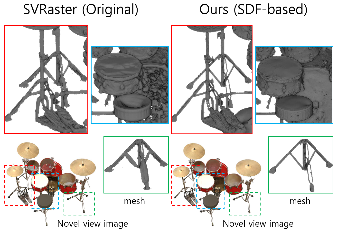
1. Motivation & Main Contribution
Motivation
- SVRaster (CVPR 2025) provides fast performance with morton code based sparse voxel rasterization, but suffers from limited geometry quality due to its density-based representation.
- NeuS (NeurlPS 2021) achieves high-fidelity geometry using SDF-based surface rendering, but is computationally heavy and not real-time friendly.
- Neuralangelo (CVPR 2023) introduced numerical eikonal loss and second-order derivative regularization to suppress noise and produce smoother surfaces.
This work integrates SDF-based learning into the SVRaster framework to improve geometry quality while preserving rasterization efficiency. Moreover, our method achieves training time less than 10 minutes, does not require SfM initialization unlike Gaussian-based approaches, and provides balanced performance: preserving novel view rendering quality, improving geometry fidelity, and extreme high rendering speed.
Main Contributions

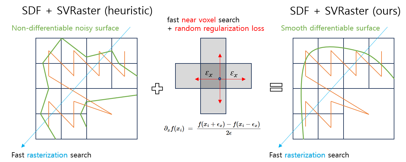
- Extension of SVRaster density mode: Added
density_mode='sdf'to apply NeuS-style $\alpha$ formulation. -
Voxel refinement improvement: Introduced SDF value criteria into subdivision and pruning to refine voxels near surfaces and prune irrelevant regions.
- Grid-Voxel mapping tables:
- Motivation: In order for regularization losses (e.g., Eikonal, smoothness) to propagate continuously across neighboring voxels, we discretize the scene into grids and enable fast neighbor queries.
- Implemented structures:
- Dense 3D bitmask (grid validity)
- Compact index table (valid grid idx list)
- Mapping table (grid idx $\rightarrow$ voxel idx, unique)
- Implemented with CUDA for efficient neighbor queries.
- Extended Loss Functions:
- Eikonal loss (numerical gradient norm $\approx 1$)
- Second-order smoothness loss (Neuralangelo-style Laplacian/Hessian $=0$)
- Random sampling loss: loss terms evaluated not only at grid centers but also at random positions within grid cells, improving convergence and reconstruction sharpness.
2. Methodology
2.1 SDF Learning within Sparse Voxels
We extend the SVRaster framework to support Signed Distance Functions (SDFs) as the scene representation.
- Each voxel maintains an implicit SDF field defined at its corner grid coordinates.
- For a ray intersecting a voxel, we compute entry and exit points ($t_{\text{entry}}, t_{\text{exit}}$), evaluate the SDF at these positions, and apply the NeuS closed-form $\alpha$ formulation:
where $\Phi_s$ is the logistic CDF and $f(\cdot)$ is the SDF.
- During backpropagation, we store the first surface hit $sdf0_t$ to compute gradients for normals and depth, and distribute these gradients to the eight voxel corners by trilinear weights.
2.2 Voxel Refinement with SDF Criteria
Sparse voxels are adaptively subdivided or pruned during training.
- Subdivision: A voxel is split into eight smaller voxels if its SDF values indicate the presence of a surface crossing (i.e., sign changes across corners or small absolute values).
- Pruning: Voxels with all SDF values consistently far from zero are removed to save computation.
- This ensures that refinement is focused only on surface-relevant regions.
- In practice, we limit the maximum subdivision depth to 2^9 (=512 grid cells per axis), since higher resolutions bring little benefit for mesh extraction while incurring heavy computational cost.
2.3 Grid–Voxel Mapping and Neighbor Search
To enable continuous propagation of regularization losses (e.g., Eikonal, smoothness, Laplacian) across space, we introduce a three-part data structure that explicitly links grid cells (fine resolution sampling points) with voxels (coarse sparse blocks). This mapping allows the system to efficiently query spatial neighbors and enforce differential constraints.
Data Structures
-
Dense Bitmask (A):
- A boolean array of size G^3 (G=2^n, where n is the maximum subdivision level) marking whether each grid coordinate is covered by any voxel.
- Acts as a global occupancy mask for the grid, enabling O(1) checks of whether a location is valid.
-
Compact Index Table (B):
- A linear array storing only valid grid indices in ascending order.
- Built from (A) using prefix-sum compaction, ensuring memory efficiency while retaining ordering.
- Querying the position of a grid index within this table requires binary search, yielding O(log M) time (where M is the number of valid grid cells).
-
Voxel Index Mapping (C):
- For each valid grid index in (B), we store the voxel index that owns this grid point.
- Each grid cell belongs to exactly one voxel, guaranteeing uniqueness and avoiding conflicts.
- This property holds because the grid is defined at the finest voxel resolution: larger voxels are subdivided into multiple smallest grid cells, so no grid cell can overlap two different voxels.
- Retrieval from this mapping is O(1) once the compacted index is known.
Neighbor Query
-
Given a grid coordinate:
- Validity Check: Query (A) -> O(1).
- Index Localization: If valid, binary search (B) to find the compacted position -> O(log M).
- Voxel Retrieval: Use (C) to obtain the corresponding voxel index -> O(1).
- Therefore, fetching the 6 neighbors of a grid coordinate costs O(6 log M) ~ O(log M).
- On the GPU, these queries are executed in parallel across thousands of threads, so in practice the effective cost approaches constant time.
Advantages
- Loss Propagation Continuity: Ensures that regularization terms applied at the grid level naturally propagate across voxel boundaries.
- GPU Efficiency: Combination of dense mask and compacted table balances memory usage (sparse storage) with parallel-friendly random access.
- Scalability: While voxels are stored adaptively and sparsely, the dense grid is always defined at the finest subdivision level. This independence allows fine-grained regularization to be applied consistently, even in regions represented by large voxels.
2.4 Loss Functions
We design two core losses, both computed per valid grid index in parallel, using finite differences.
(a) Eikonal Loss (numerical gradient)
We enforce the gradient norm of the SDF to be close to 1.
For each grid coordinate $x_i$, the gradient is approximated by central differences:
Then the loss is
\[L_{\text{eik}} = \frac{1}{N}\sum_{i=1}^N \Bigl|\,\|\nabla f(x_i)\|_2 - 1\,\Bigr|.\](b) Smoothness Loss (second-order Laplacian)
We regularize the second derivatives so that curvature vanishes, similar to Neuralangelo.
At each grid coordinate $x_i$, the Laplacian is estimated with second-order finite differences:
The smoothness loss is then
\[L_{\text{smooth}} = \frac{1}{N}\sum_{i=1}^N \bigl|\,\nabla^{2} f(x_i)\,\bigr|.\](c) Random Sampling within Grid Cells
Both eikonal and smoothness losses are also evaluated at random positions inside each grid cell:
\[x' = x + \delta,\qquad \delta \sim \mathcal{U}(0.0, 1.0)\cdot h\]where $h$ is the grid spacing.
This stochastic sampling improved stability and resulted in sharper and less noisy geometry in our experiments.
3. Experimental Results
3.1 Qualitative Results
(a) Novel View Synthesis Comparison
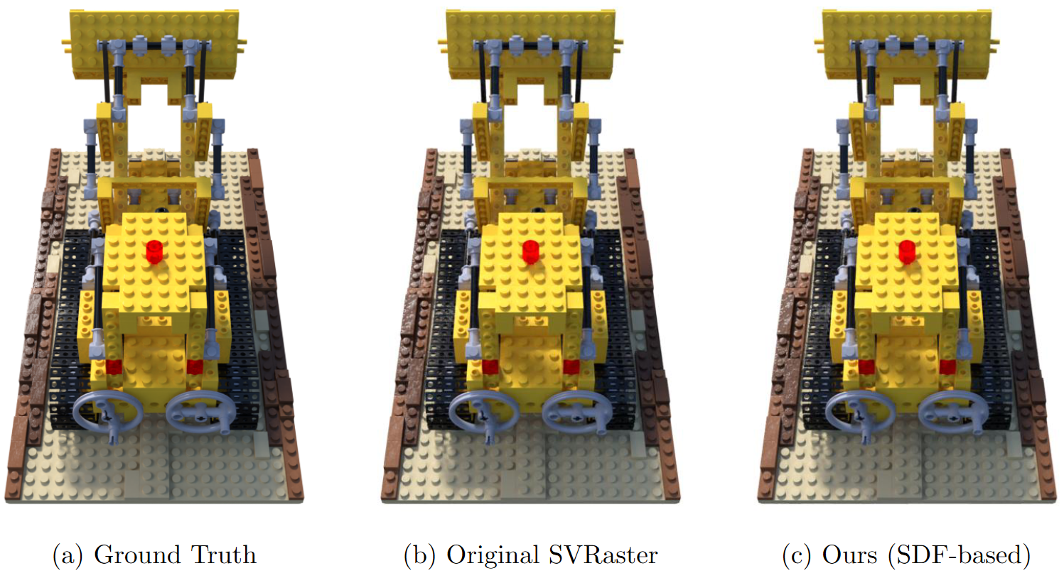
Our method preserves novel view rendering quality comparable to the original SVRaster, while providing improved geometry.
(b) Geometry Comparison with Original SVRaster
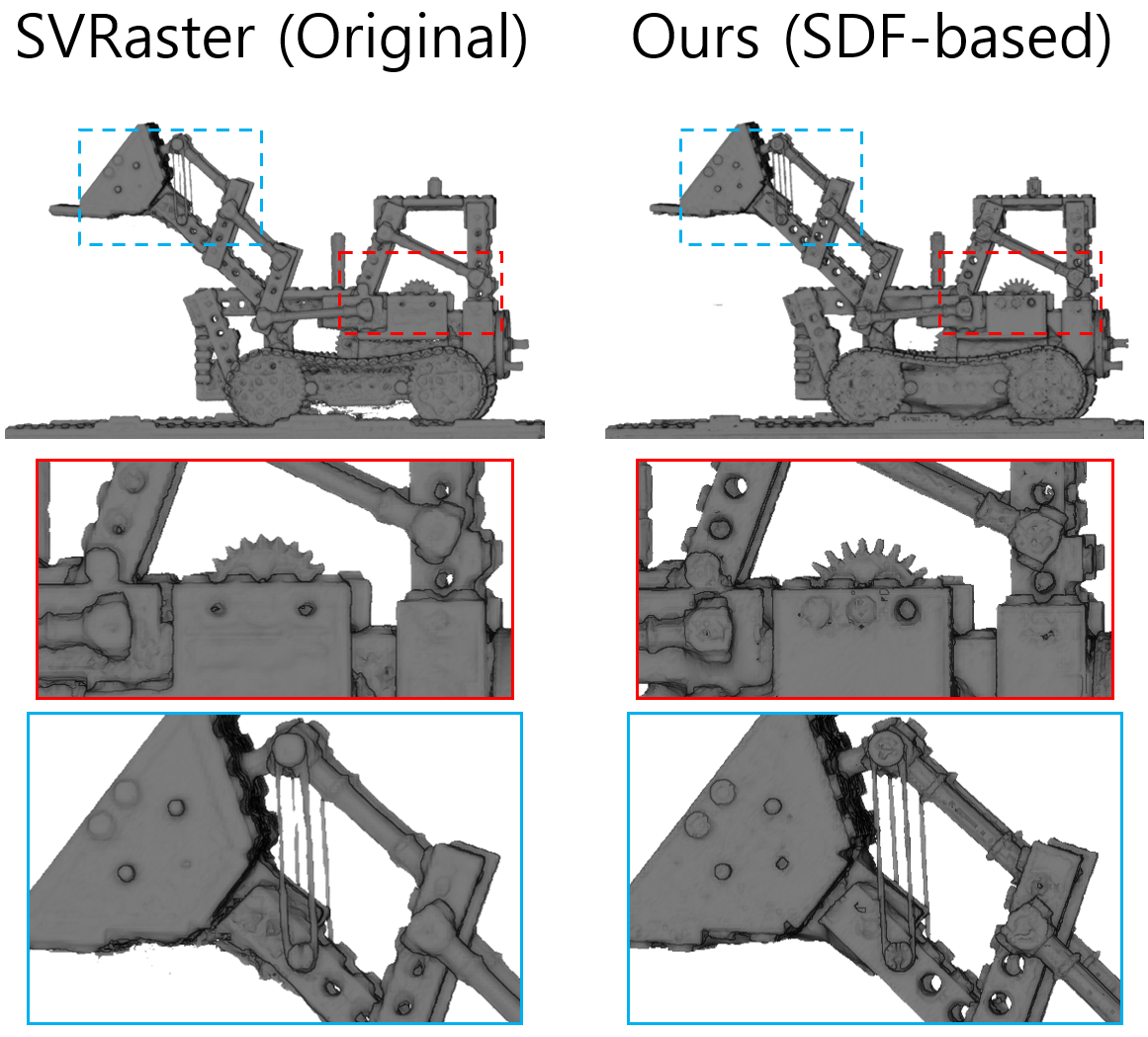
Compared to the original SVRaster, our SDF-based method captures finer structures and represents geometry with higher fidelity.
(c) Ablation: Effect of Random Sampling for Regularization
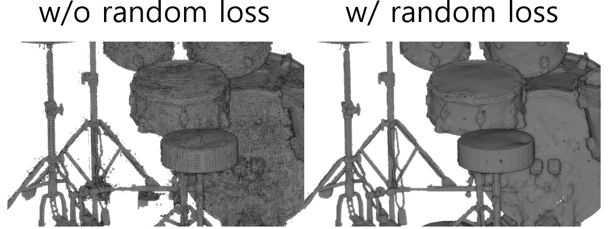
Random sampling inside grid cells reduces noise and improves surface smoothness.
3.2 Quantitative Results
We evaluated Chamfer Distance on the DTU dataset (lower is better).
The table below highlights our reproduced result compared to the original SVRaster and other baselines.
| Method | DTU (scan 24) Chamfer Distance |
|---|---|
| NeuS | 1.00 |
| 2DGS | 0.48 |
| 3DGS | 2.14 |
| SVRaster (original, density) | 0.61 |
| Ours (reproduced) | 0.52 |
- Our reimplementation achieves 0.52, which improves upon the reported SVRaster (0.61) and is consistent with the relative ranking of methods.
Results Summary
Our method provides a balanced set of advantages:
- Novel view rendering: quality on par with original SVRaster.
- Geometry fidelity: significantly improved, approaching NeuS/Neuralangelo.
- training, Rendering speed: training converges in under 10 minutes and inference runs at real-time rasterization rates.
- Initialization: no SfM is required, unlike Gaussian-based methods.
Together, these results show that our approach combines the strengths of rasterization, SDF-based learning, and efficiency, without being dominated by any existing category of methods.